flowchart TB
  subgraph T["XGBoost / LightGBM: train, then predict"]
    direction LR
    A["Training rows<br/>+ labels"] --> B["Fit hundreds of trees<br/>(+ tuning)"]
    B --> C["New model for<br/>this dataset"]
    D["Test rows"] --> C
    C --> E["Predictions"]
  end
  subgraph K["Kumo Tabular: in-context learning"]
    direction LR
    F["Training rows<br/>+ labels"] --> H["Frozen pretrained transformer<br/>one forward pass, no weight updates"]
    G["Test rows"] --> H
    H --> I["Predictions"]
  end
  T ~~~ K
Can a pretrained model beat XGBoost without training?
NVIDIA Kumo Tabular vs gradient-boosted trees, plus a rematch with my 2020 Bank Marketing models
tabular
foundation models
in-context learning
xgboost
benchmarking
With zero tuning, NVIDIA’s Kumo Tabular beat default XGBoost and LightGBM on 25 of 25 splits, won most on small data, and edged out my hand-tuned 2020 models on Bank Marketing. Rebuilding those 2020 models also exposed a train/test leak.
 Full notebook with outputs · Code and data on GitHub
NoteTL;DR
- With zero tuning, NVIDIA Kumo Tabular beat default XGBoost and LightGBM on 25 of 25 train/test splits across five OpenML datasets, by +0.034 ROC-AUC on average.
- The advantage is largest with little data. On adult it was +0.05 ROC-AUC at 100 training rows and +0.01 at 10,000.
- On Bank Marketing it edged out my hand-tuned 2020 models. It had the best PR-AUC both with the leaky
durationfeature (0.566 vs 0.542 for tuned XGBoost) and without it (0.373 vs 0.349). - Rebuilding the 2020 models exposed a bug in my 2020 notebook. Its random forest scores look inflated by train/test leakage.
- The cost is speed. On a 10k-row table Kumo large took about 80 s on a T4 GPU, while XGBoost took 0.3 s on CPU. Kumo small was nearly as accurate at about 11 s.
The question
Gradient-boosted trees have been the default answer for tabular data for a decade. Tabular foundation models take a different route, and NVIDIA’s Kumo Tabular reports first place on the TabArena and TALENT benchmarks.
I wanted to check two things on a free Colab GPU:
- With zero tuning, does it beat default XGBoost and LightGBM on small and medium classification tables?
- How does it compare with the hand-tuned models from a Bank Marketing notebook I wrote in 2020?
How in-context learning works
A gradient-boosted tree model is trained. You give it your training rows, it builds hundreds of trees to fit them, and you then use those trees to predict new rows. Every dataset gets its own freshly fitted model, usually with hyperparameter tuning on top.
Kumo Tabular is never trained on your data. Its weights were fixed once, by NVIDIA, after pretraining on tens of millions of synthetic tables. The tables were generated from random causal graphs, so the model has seen a huge variety of “features cause a target” patterns, but no real dataset. To make a prediction, you pass it two things in a single forward pass:
- your labelled training rows (the context), and
- the unlabelled rows you want predictions for (the queries).
Inside the transformer, each query row attends to the context rows and their labels and infers the relationship on the fly, much as an LLM picks up a task from worked examples in its prompt. Nothing is fitted, nothing is tuned and no weights change. The “learning” happens inside one forward pass, which is why it’s called in-context learning (ICL).
| XGBoost / LightGBM | Kumo Tabular (ICL) | |
|---|---|---|
| Uses your training rows | to fit a new model | as context in a forward pass |
| Weights change? | yes, built from scratch per dataset | no, frozen after pretraining |
| Hyperparameter tuning | usually needed | none |
| What it learned beforehand | nothing | priors from ~35–137M synthetic tables |
| Compute | cheap CPU | GPU; cost grows with context size |
| Practical limit | none really | context size (here 10k rows per ensemble member) |
So this isn’t zero-shot. The model needs labelled examples, and in every comparison here it gets exactly the same training rows as XGBoost and LightGBM. It’s zero-training. The pretrained prior is what lets it do well from very few rows.
Setup
| Part | What | Models |
|---|---|---|
| A | 5 OpenML-CC18 binary datasets × 5 stratified 75/25 splits (train capped at 10k rows, test at 5k) | XGBoost (default), LightGBM (default), TabICLv2, Kumo Tabular small (28M params) and large (215M) |
| Learning curve | adult and Bank Marketing (no duration), 100 to 10k training rows, 3 seeds |
XGBoost, LightGBM, Kumo Tabular large |
| B | UCI Bank Marketing on the 2020 split and encoding, with and without the leaky duration feature |
The four 2020 models, rebuilt with their 2020 tuned hyperparameters, plus all Part A models |
| Controls | Leak check for the 2020 numbers; shuffled-label check for the in-context models | as above |
- No tuning anywhere except the 2020 models, which keep their 2020 tuned settings. The GBDTs use library defaults with native categorical handling.
- Kumo settings: 8 ensemble members, fp16, at most 10k context rows per member.
- Hardware: Colab T4 GPU for the in-context models, Colab’s 2 vCPUs for the trees.
- Reproducibility: a full rerun reproduced every Part A ROC-AUC to 4 decimal places.
TipGetting it installed
Kumo Tabular ships in NVIDIA’s structured-data-models library, which is still alpha. Two traps:
pip install structured-data-modelsinstalls an empty0.0.0a0placeholder, even though the Hugging Face model card suggests it. Install from GitHub instead. The notebook pins commitce95710.- The code snippet in NVIDIA’s blog post has typos (
pd.load_csv,drop_column). Follow the repo’s own examples instead.
The weights download from Hugging Face without a token, and everything runs on a free Colab T4.
Results
Part A: five OpenML datasets, 5 splits each
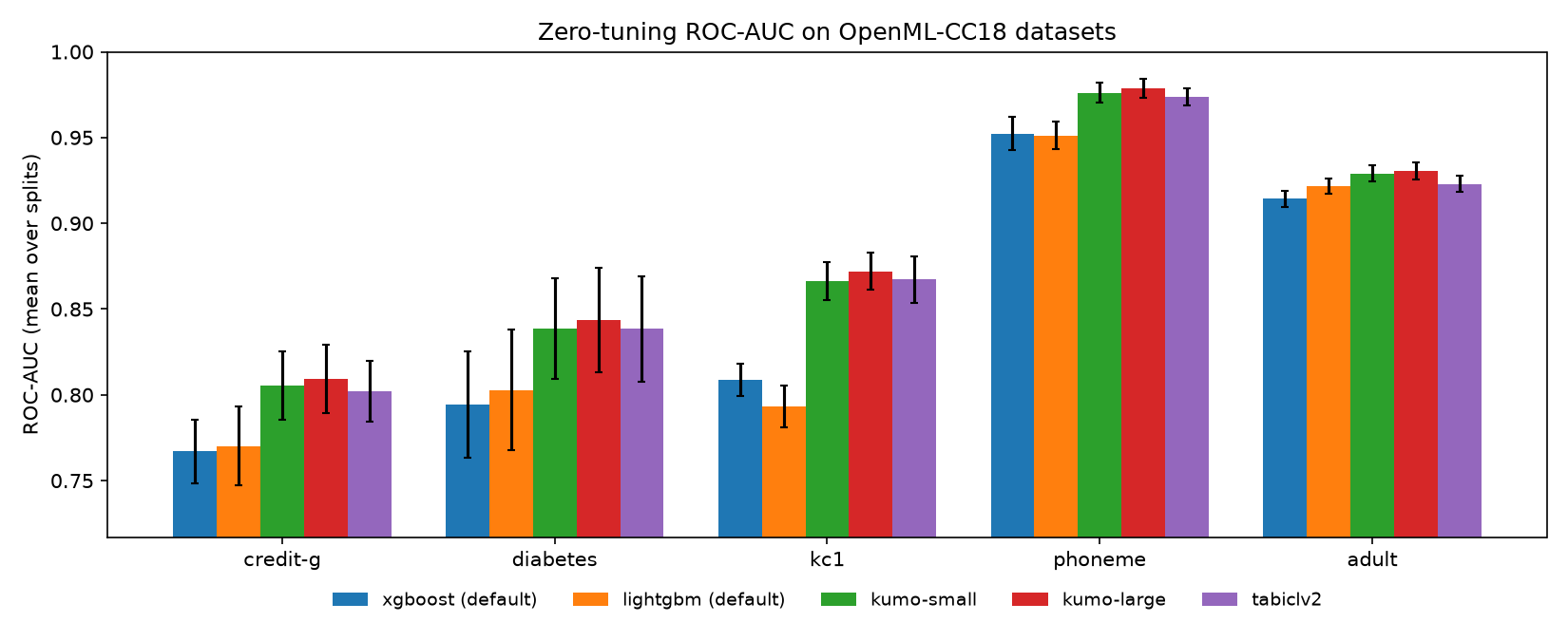
Mean ROC-AUC over 5 splits:
| Dataset | Rows | XGBoost | LightGBM | TabICLv2 | Kumo small | Kumo large |
|---|---|---|---|---|---|---|
| credit-g | 1,000 | 0.767 | 0.770 | 0.802 | 0.805 | 0.809 |
| diabetes | 768 | 0.794 | 0.803 | 0.838 | 0.839 | 0.843 |
| kc1 | 2,109 | 0.809 | 0.793 | 0.867 | 0.866 | 0.872 |
| phoneme | 5,404 | 0.952 | 0.951 | 0.974 | 0.976 | 0.979 |
| adult | 48,842 | 0.914 | 0.922 | 0.923 | 0.929 | 0.930 |
| Mean rank | 4.52 | 4.44 | 2.72 | 2.24 | 1.08 |
- Kumo large beat the better of the two GBDTs on 25 of 25 splits, by +0.034 ROC-AUC on average. Its smallest margin was +0.007.
- Kumo small also won 25/25 (+0.030). TabICLv2 won 24/25, with one tie (+0.028).
- The gap was largest on the smaller tables (kc1 +0.06, diabetes +0.04, credit-g +0.04) and smallest on adult (+0.008).
- The in-context models were also better calibrated. Default XGBoost’s log loss was about 1.5× Kumo large’s on credit-g (0.70 vs 0.47) and on diabetes (0.75 vs 0.46).
Learning curve: the less data, the bigger the win
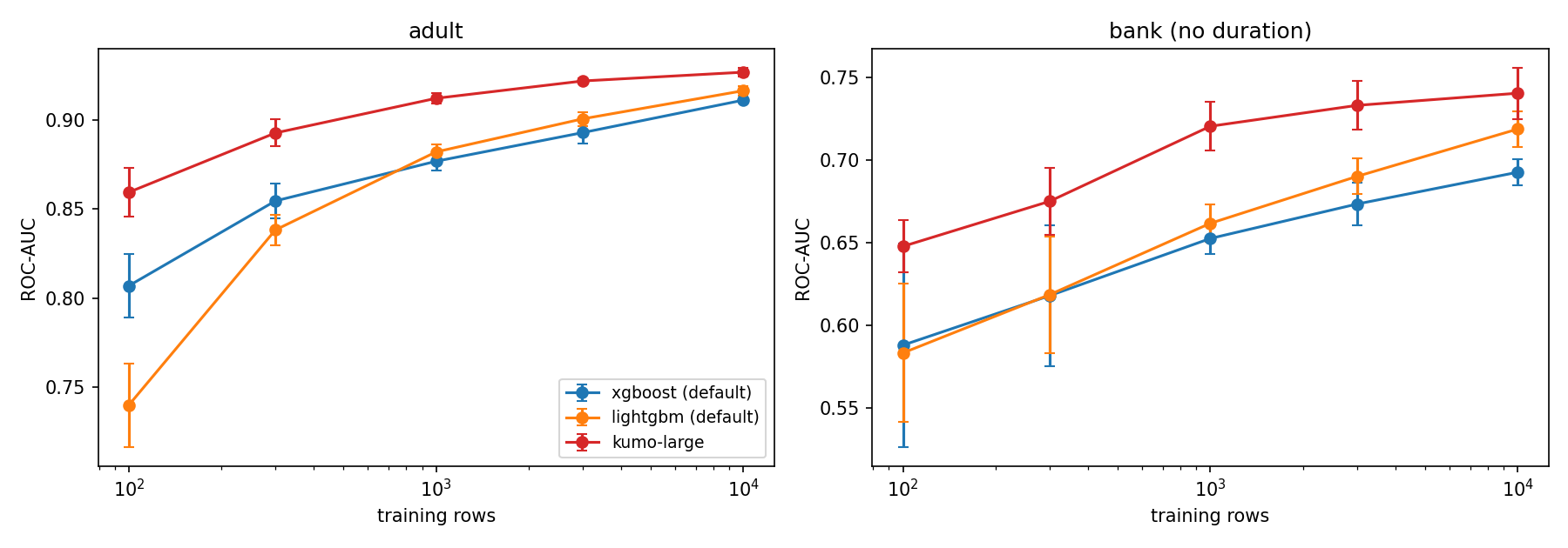
Mean ROC-AUC over 3 seeds:
| Dataset | Training rows | XGBoost | LightGBM | Kumo large |
|---|---|---|---|---|
| adult | 100 | 0.807 | 0.740 | 0.859 |
| adult | 1,000 | 0.877 | 0.882 | 0.912 |
| adult | 10,000 | 0.911 | 0.917 | 0.927 |
Bank Marketing (no duration) |
100 | 0.588 | 0.584 | 0.648 |
Bank Marketing (no duration) |
1,000 | 0.653 | 0.662 | 0.720 |
Bank Marketing (no duration) |
10,000 | 0.693 | 0.719 | 0.740 |
- Kumo large led at every training size, and its lead shrank as data grew.
- It needed far fewer rows to match the trees. On Bank Marketing, Kumo with 1,000 rows matched the best GBDT with 10,000 rows (0.720 vs 0.719). On adult it needed 3,000 rows (0.922 vs 0.917).
Part B: a rematch with my 2020 Bank Marketing models
Test set: 9,043 rows, 11.7% positive.
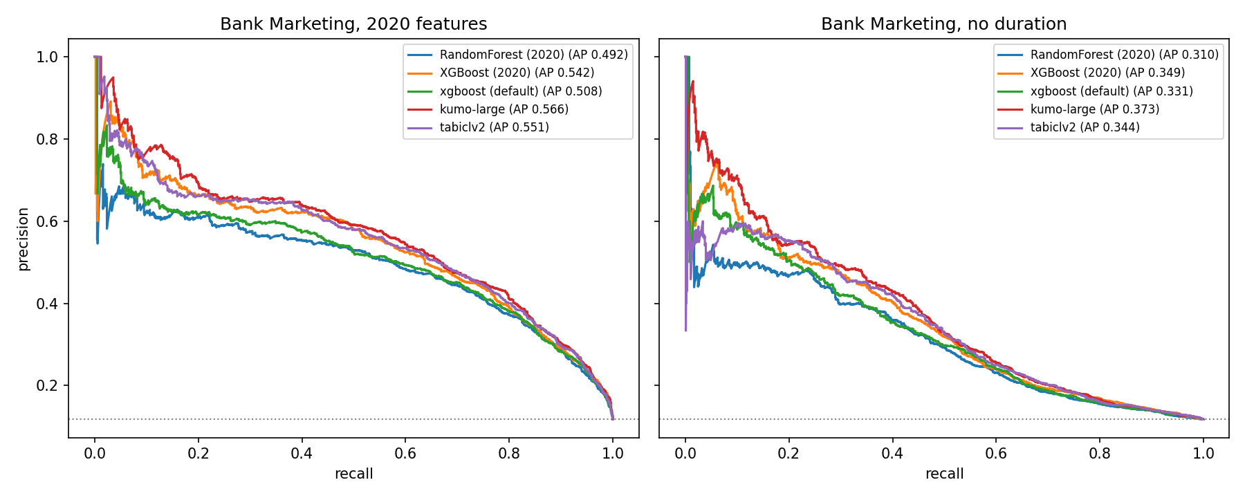
The 2020 notebook kept duration (call length). UCI warns against using it for a realistic model, because you only know it once the call is over. So Part B runs twice: once with the 2020 feature set (like for like) and once without duration (the honest task).
| Model | 2020 features: ROC-AUC | 2020 features: PR-AUC | No duration: ROC-AUC |
No duration: PR-AUC |
|---|---|---|---|---|
| Logistic regression (2020) | 0.860 | 0.466 | 0.690 | 0.268 |
| Logistic regression + SMOTE (2020) | 0.864 | 0.468 | 0.691 | 0.269 |
| Random forest + SMOTE (2020) | 0.885 | 0.492 | 0.715 | 0.310 |
| XGBoost, tuned and cost-sensitive (2020) | 0.895 | 0.542 | 0.733 | 0.349 |
| XGBoost (default) | 0.888 | 0.508 | 0.722 | 0.331 |
| LightGBM (default) | 0.897 | 0.540 | 0.740 | 0.351 |
| TabICLv2 | 0.898 | 0.551 | 0.737 | 0.344 |
| Kumo small | 0.900 | 0.564 | 0.737 | 0.356 |
| Kumo large | 0.901 | 0.566 | 0.739 | 0.373 |
- Kumo large had the highest PR-AUC in both variants, with zero tuning. It beat the 2020 XGBoost, which took about 8 minutes of random search, by +0.024 in both variants. Without
duration, ROC-AUC is effectively a tie with default LightGBM (0.739 vs 0.740). durationwas doing most of the work. Removing it cost every model 0.16–0.17 ROC-AUC, so much of my 2020 notebook’s apparent skill came from a feature that isn’t available at prediction time.- At a 0.5 threshold the picture differs. Kumo large with
durationgets precision 0.64, recall 0.40 and F1 0.49. The 2020 random forest (SMOTE) gets 0.44, 0.71 and 0.54. Nothing tells the in-context models about the 88/12 class imbalance, so they predict “yes” conservatively, whereas SMOTE andscale_pos_weightdeliberately trade precision for recall. Choosing the threshold from the precision-recall curve closes that gap.
My 2020 numbers don’t reproduce, and why
Rebuilt with the same split, encoding and tuned hyperparameters, the 2020 logistic regressions match what the 2020 notebook printed. The random forest and XGBoost don’t:
| F1 at threshold 0.5 | Printed in 2020 | Rebuilt today |
|---|---|---|
| Logistic regression | 0.30 | 0.33 |
| Logistic regression + SMOTE | 0.47 | 0.47 |
| Random forest + SMOTE | 0.65 | 0.54 |
| XGBoost | 0.64 | 0.51 |
The 2020 notebook shuffled the data without a seed and evaluated models loaded from .pkl files. If those pickles were trained in an earlier session, that session had a different shuffle. A large share of the 2020 “test” rows would then have been training rows for the pickled models.
Simulating exactly that (train on one shuffle’s split, score on another shuffle’s test split):
| Model | F1, clean test | F1, reshuffled test | Printed in 2020 |
|---|---|---|---|
| Logistic regression | 0.32 | 0.33 | 0.30 |
| Logistic regression + SMOTE | 0.49 | 0.49 | 0.47 |
| Random forest + SMOTE | 0.54 | 0.68 | 0.65 |
| XGBoost | 0.53 | 0.55 | 0.64 |
- Random forest: the leak reproduces its 2020 numbers almost exactly (precision 0.56 vs 0.54, recall 0.86 vs 0.84). A depth-16 forest memorises its training rows, so leaked rows inflate its score.
- Logistic regression: unaffected, as you’d expect from a model that can’t memorise.
- XGBoost: the leak explains only a small part of its gap; the rest is unexplained.
My 2020 random forest was most likely never as good as the notebook reported.
Did Kumo just memorise these datasets?
All six datasets are well-known public benchmarks. Kumo Tabular is reportedly pretrained only on synthetic tables, but it’s fair to ask whether its edge comes from having effectively “seen” these datasets before.
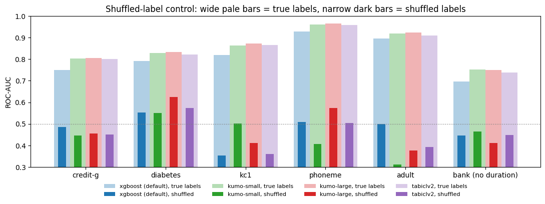
To test that, each model got the same training rows with randomly permuted labels: same class balance, no real relationship to the features. A model that learns from its context should fall to chance (ROC-AUC ≈ 0.5). One that recognises the dataset would keep scoring well.
| Model | Mean ROC-AUC, true labels | Mean ROC-AUC, shuffled labels |
|---|---|---|
| Kumo large | 0.858 | 0.475 |
| Kumo small | 0.855 | 0.446 |
| TabICLv2 | 0.849 | 0.455 |
| XGBoost (default) | 0.814 | 0.474 |
- Every model collapsed to chance or below, and the in-context models collapsed as fully as XGBoost, which can’t have memorised anything.
- Individual runs are noisy (0.25–0.66), XGBoost included.
- No sign of memorisation. The performance comes from the labelled rows in context.
What it costs
Median fit-plus-predict time per split:
| Dataset | XGBoost (CPU) | LightGBM (CPU) | TabICLv2 (T4) | Kumo small (T4) | Kumo large (T4) |
|---|---|---|---|---|---|
| credit-g (750 train / 250 test) | 0.09 s | 0.06 s | 0.39 s | 0.55 s | 1.2 s |
| phoneme (4k / 1.4k) | 0.12 s | 0.12 s | 0.97 s | 0.85 s | 7.3 s |
| adult (10k / 5k) | 0.31 s | 0.20 s | 11.0 s | 10.6 s | 80.7 s |
On adult, Kumo large was about 250× slower than XGBoost and Kumo small about 35× slower. Kumo small gave up only 0.004 ROC-AUC on average for an 8× speed-up over large, so on this evidence it’s the better default.
What I take from this
- For small and medium tables, a pretrained in-context model is now a strong default. With no tuning, Kumo Tabular beat untuned GBDTs on every split I tested, often by a margin bigger than the split-to-split noise. On Bank Marketing it also beat my tuned 2020 XGBoost on PR-AUC.
- The less data you have, the bigger the win. Kumo needed roughly 3–10× fewer rows than the trees to reach the same ROC-AUC. As data grows towards the context limit, the GBDTs close in.
- Kumo small is the practical choice. It came within 0.004 ROC-AUC of large at about one-eighth of the cost.
- Thresholds still need thought. The in-context models aren’t told about class imbalance, so on imbalanced problems pick the operating point from the precision-recall curve rather than using 0.5.
- The rematch was most useful for checking my old work. It surfaced a leaky feature (
duration) and a train/test leak that likely inflated my 2020 random forest results.
Limitations
- Small benchmark. Five binary datasets and one extra case study. NVIDIA’s claims rest on TabArena’s 51 datasets. These results are a sanity check on public data, not a ranking.
- Untuned baselines. Except for the 2020 models, the GBDTs ran at library defaults with no early stopping. Tuned GBDTs would close some of the gap.
- Context cap. Kumo saw at most 10k training rows per ensemble member, and used 8 members rather than the 16 in NVIDIA’s benchmark.
- Public datasets. The shuffled-label control rules out memorisation of these datasets, but it can’t rule out that the model’s design was tuned on public benchmarks like these. A dataset published after the model, or private data, would be a stronger test.
- Timing compares a GPU with a 2-vCPU CPU. It reflects practical cost on free Colab, not algorithmic efficiency.
- Fine-tuning not tested. Every Kumo number here is from the frozen pretrained model.
Data and reproducibility
| Dataset | Source | Licence |
|---|---|---|
| credit-g, diabetes, kc1, phoneme, adult | OpenML 31, 37, 1067, 1489, 1590 | Public |
Bank Marketing (bank-full.csv) |
UCI 222 | CC BY 4.0 |
Bank Marketing: S. Moro, P. Cortez and P. Rita (2014), A Data-Driven Approach to Predict the Success of Bank Telemarketing, Decision Support Systems 62:22–31.
Everything, including setup, every table, every chart and the controls, is in the full notebook. It runs top to bottom on a free Colab T4 with the Open in Colab button. The raw results CSVs are on GitHub.